Machine Learning
There are three main types of algorithms distinguished by their learning style:
Supervised Learning, Unsupervised Learning, and Semi-Supervised Learning.
Supervised Learning, Unsupervised Learning, and Semi-Supervised Learning.
Semi-Supervised Learning is a mixture of labelled and unlabelled input data that requires some learning of structures as well as some predictions. (Ex. Regression, Classification) |
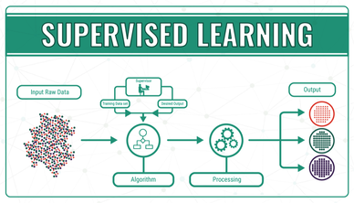
Supervised Learning creates an environment where a labeled training set is given and a machine is allowed to make predictions based on the input data. Machines will correct predictions until accuracy reaches a reasonable level, which will allow for generalizations based on the training data. (Ex. Regression, Classification)
|
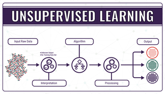
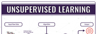
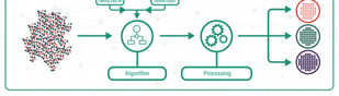
Unsupervised Learning gives an unlabeled input set and allows the machine to deduce hidden structures by grouping elements through general rules.(Ex. Clustering, Association rule learning)
|
Types of Methods:
Regression: Predicting a particular numerical value based on a set of prior data. (Ex. regularized linear regression, polynomial regression, decision trees and random forest regressions)
Classification: Classification methods predict a class value based on input data. (Ex. Decision Trees)
Clustering: Cluster observations with similar characteristics and let the algorithm predict output. (Ex. K-means)
K-means brief explanation: Chooses K amount of centers within a particular data set and assigns each data point to the closest center. Then, recalculates the cluster centers.
Others:Dimensionality Reduction, Natural Language processing, Neural nets
Neural Network (inspired by biological networks in the human brain)
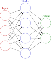
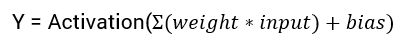
Neural Networks are a type of Supervised Machine Learning, which can exist as convolutional neural networks (image recognition/classification)(CNNs) or recurrent neural networks (sequential representation)(RNNs). In a neural network there exists a bias, a trainable constant provided to every node that is used to adjust the output so it will have a better prediction in the end along with a weight.
Within the hidden nodes there exists activation functions( ex. ReLu, Sigmoid, Binary Step) which introduce non linearity and acts as the transfer between input and output.
Within the hidden nodes there exists activation functions( ex. ReLu, Sigmoid, Binary Step) which introduce non linearity and acts as the transfer between input and output.
Where the training comes in is the back propagation algorithm; error is propagated to the previous layer, and "learns from its mistakes", then proceeds repeat the process until the output error is less than a certain threshold.
Combining Machine Learning and Materials Science
One of the many uses of machine learning is predicting the behaviors/properties of different materials given a test data set. In our project to predict the poisson ratio and elastic anisotropy of a given material, we used Pycharm 3.0 to gather databases from matminer to begin the process to train our model.
To begin with, we will start by attempting to train a model to predict the elastic anisotropy of a material. Anisotropy is defined as the property of having directional dependance, which will lead to an exhibition of varying properties along different directions. Elastic Anisotropy will determine a material's anisotropy of elastic properties.
Within Pycharm 3.0, it is important to first install the numpy, matplotlib, and matminer packages within the project interpreter in your venv(virtual environment).
The next step is to import some very useful databases and functions to allow our program to access the internet for assistance in plotting, processing, etc.
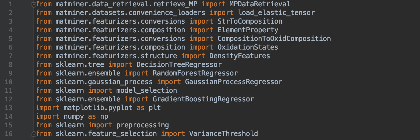
As a note, these sklearn imports for regressors are up to the user to decide which regressors to test and use.
The next step is to create the database and commence the data exploration.
The next step is to create the database and commence the data exploration.
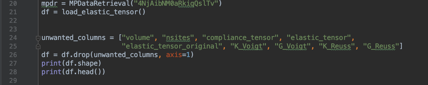
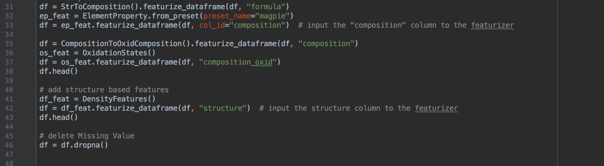
Here, we are getting rid of any columns that do not contain float values, as we will be testing for floats and not any other type of variable. While experimenting with this, we found that if these columns remain, then there will be an error when running the program, so it is essential for all features to be of the float type. By printing out the shape and head of the database, we are able to get a visualization of what the table actually looks like, a step that should always be performed before any training begins.
We will now add some features to the database to get the most optimal prediction out of a large variety.
We will now add some features to the database to get the most optimal prediction out of a large variety.
Now, we will add some data processing to help our model get a better estimate.
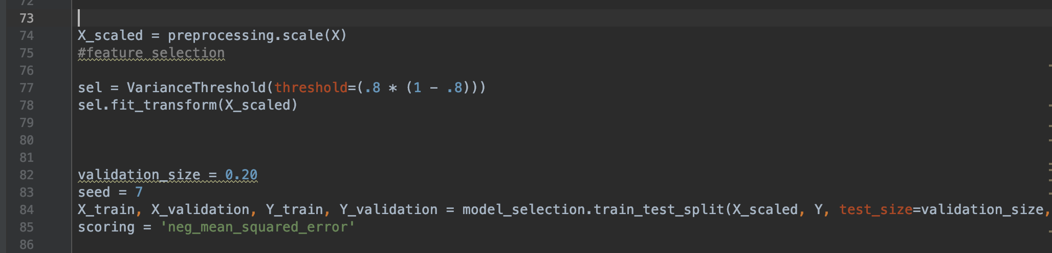
The preprocessing.scale() is a type of standardization that is essential for machine learning because the model must look Gaussian with zero mean and unit variance to get a good estimate. What the VarianceThreshold() does is remove all variance that doesn't meet the threshold in order to process out the outliers that may mess up the accuracy of the model.
In order to train the model, we will set aside 20% of our database as the "training" set, which would represent supervised input, and keep 80% to predict. This is where the train_test_split() method comes in, which will split our data into X_train, Y_Train, X_Scaled, and Y.
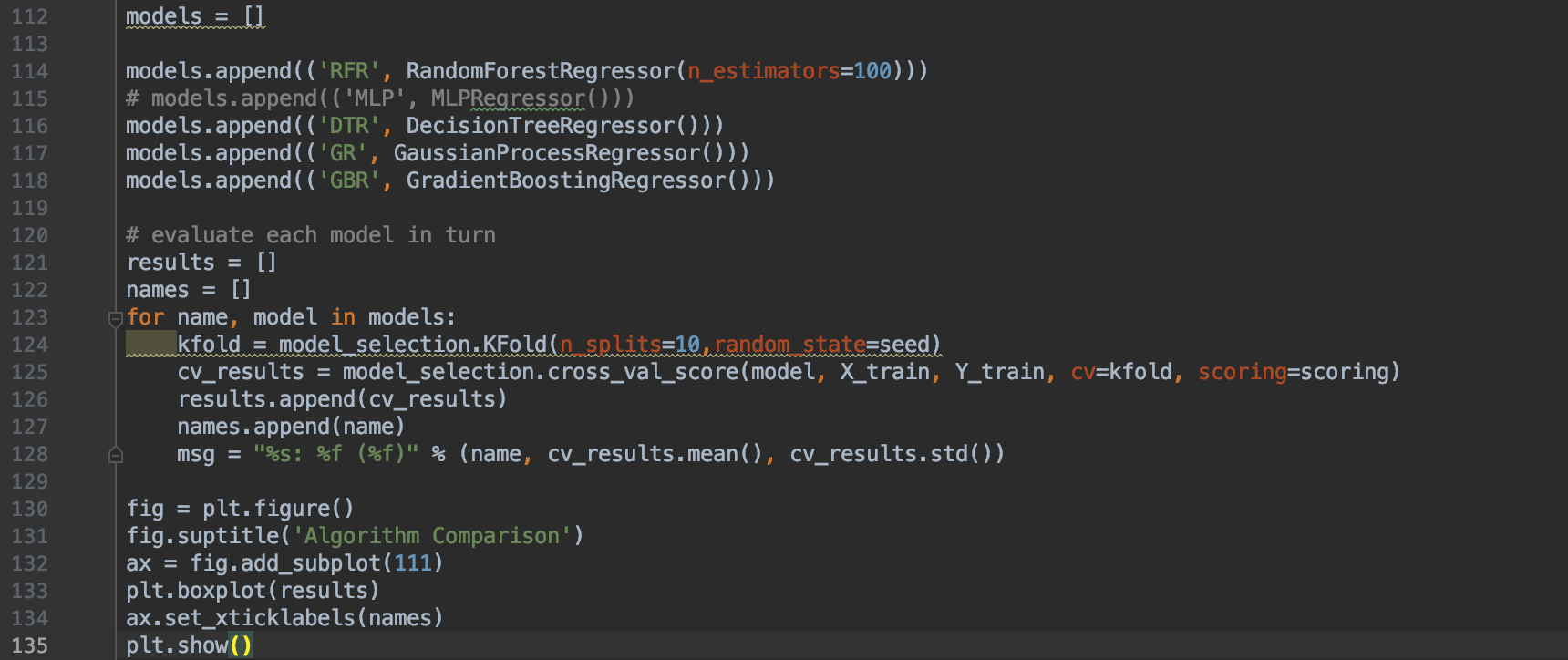
To test out which regression method we will use, we will test the negative mean squared error of each method and choose the one with the least error to proceed with.
In order to train the model, we will set aside 20% of our database as the "training" set, which would represent supervised input, and keep 80% to predict. This is where the train_test_split() method comes in, which will split our data into X_train, Y_Train, X_Scaled, and Y.
To test out which regression method we will use, we will test the negative mean squared error of each method and choose the one with the least error to proceed with.
Careful of overfit
